Tutorials

Tutorial 1: A single, flat interface

In this example, we compute the reflection and transmission coefficients at a single, flat interface between a superstrate (incident medium) and a substrate. The example file can be found is under examples/FresnelCoefficients.py. The simulation can be run either in two or three dimensions, to demonstrate the syntax adjustments in creating the S⁴ simulation object.

Once S4 has been installed, you should be able to import it, along with numpy and matplotlib.pyplot:

import S4 as S4
import numpy as np
import matplotlib.pyplot as plt

As stated in the S4 documentation, “S⁴ solves the linear Maxwell’s equations, which are scale-invariant. Therefore, S⁴ uses normalized units, so the conversion between the numbers in S4 and physically relevant numbers can sometimes be confusing.” In order to clearly link the reduced units and the actual physical ones, we keep track of the speed of light (assumed to be 1 in S⁴):

c_const = 3e8

and the general scale is defined by the period of the lattice:

a = 1 ## period, normalized units. This defines the length scale

So if we (arbitrarily) decide that a here is in units of micrometers, we can run the simulation at a wavelength of 1 micron by setting the following:

lbda = 1e-6 ## say we compute at 1µm wavelength
f = c_const/lbda ## ferquency in SI units
f0 = f/c_const*1e-6 ## so the reduced frequency is f/c_const*a[SI units]

We pick the dimension of the simulation (2 or 3), then we set the lattice period and the number in-plane Fourier expansions order to be used (S4.New):

Dimension = 3 # 2 or 3

if Dimension == 2:
    ### 2 dimensional simulation, 1D lattice
    S = S4.New(Lattice = a,
                NumBasis = 1)
elif Dimension == 3:
    ### 3 dimensional simulation, 2D lattice
    S = S4.New(Lattice = ((a,0), (0,a)),
                NumBasis = 1)

In the case of a 2D simulation, the lattice is one-dimensional and has a simple period a. For the 3D simulation, the lattice dimension is two and we choose a square lattice of period a in both dimensions. Since the layer is unpatterned, we only need to compute the 0^th plane wave order, and hence NumBasis=1 is enough.

We then setup the main parameters of the simulation: the angle of incidence \(\theta\), and the refractive indices of the superstrate and substrate:

theta = np.arange(0,89,2) ## angle of incidence in degree

n_superstrate = 1 ## incident medium index
eps_superstrate = n_superstrate**2 ## incicent medium permittivity
n_substrate = 2 ## substrate index
eps_substrate = n_substrate**2 ## substrate permittivity

S⁴ uses (possibly complex and anisotropic) permittivities instead of refractive index, which is used when declaring the materials used in the simulation (S.SetMaterial):

S.SetMaterial(Name='Air', Epsilon = eps_superstrate)
S.SetMaterial(Name='Substrate', Epsilon = eps_substrate)

The names used in declaring the materials ('Air' and 'Substrate') will be used to set the permittivities of the layers that we declare, setting their names and thickness (S.AddLayer):

AirThick = 1 ## in reduced units, same scale as a
SubThick = 1 ## in reduced units, same scale as a

S.AddLayer(Name='Air', Thickness=AirThick, Material='Air')
S.AddLayer(Name='Substrate', Thickness=SubThick, Material='Substrate')

The layers are added in order, from the top (incident layer) to the bottom (substrate) one.

At this point the simulation is set up, and we can now run it to retrieve the reflection and transmission coefficients. We initialize the arrays storing the results:

Rte = np.zeros(len(theta))
Rtm = np.zeros(len(theta))
Tte = np.zeros(len(theta))
Ttm = np.zeros(len(theta))

and set the (single) frequency at which the simulation runs (S.SetFrequency):

S.SetFrequency(f0)

The bulk of the calculation is in the main loop over the angle of incidence:

for ii, thi in enumerate(theta):
    ########
    ## TM excitation
    S.SetExcitationPlanewave(
            IncidenceAngles=(thi,0), #S4 names are reversed (phi,theta)
            sAmplitude=0.,
            pAmplitude=1.,
            Order=0)
    inc, r = S.GetPowerFlux(Layer='Air',zOffset=0)
    fw, _ = S.GetPowerFlux(Layer='Substrate', zOffset=SubThick)
    Rtm[ii] = np.abs(-r/inc)
    Ttm[ii] = np.abs(fw/inc)

    #########
    ## TE excitation
    S.SetExcitationPlanewave(
            IncidenceAngles=(thi,0), #S4 names are reversed (phi,theta)
            sAmplitude=1.,
            pAmplitude=0.,
            Order=0)
    inc, r = S.GetPowerFlux(Layer='Air',zOffset=0)
    fw, _ = S.GetPowerFlux(Layer='Substrate', zOffset=SubThick)
    Rte[ii] = np.abs(-r/inc)
    Tte[ii] = np.abs(fw/inc)

The exciting wave properties are set through the S4.SetExcitationPlanewave method. The arguments are the couple of incidence angles (theta,phi) in spherical coordinates which represent the polar angle and the azimuthal angle. (Note that the S4 documentation uses the opposite denomination), the amplitude of the s- and p-components of the electric field, and the order (defaults to 0, see doc). Note that here we use the enumerate function from python which allows us to pass directly the local variable thi to the plane wave function.

We use the method S.GetPowerFlux which returns the integral of the z component of the Poynting vector over unit cell surface normal to the z direction, decomposed into forward and backward propagating modes. Hence, the incident and reflected power is obtained using:

inc, r = S.GetPowerFlux(Layer='Air',zOffset=0)

so the calculation is lead in the first layer. The zOffset parameter specifies the vertical offset (in reduced units) from the front surface of the layer. This only matters for lossy layers. Conversly, the transmitted power is obtained with:

fw, _ = S.GetPowerFlux(Layer='Substrate', zOffset=SubThick)

where we discard the value of the backward propagating wave from the substrate, since it should be 0 by definition. Note that we specified a zOffset equal to the layer thickness only for the sake of clarity.

As stated in the S4 documentation, the incident power is only unity at normal incidence. Hence, the values extracted from the simulation have to be normalized by the input power:

Rtm[ii] = np.abs(-r/inc)
Ttm[ii] = np.abs(fw/inc)

(note the sign convention for the reflected power) and we take the absolute value abs to cast the (otherwise complex) value returned by the simulation to a real number.

We can plot the results and compare to the Fresnel coefficients formula, as well as the Brewster angle:

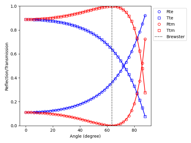
where the symbols are the results of the simulations, and the solid lines the analytical results.

Tutorial 2: A single slab, or Fabry-Pérot etalon

We now quickly move on to a similar, simple example demonstrating the calculation of the transmission and reflection from a single dielectric slab, either as a function of angle of incidence or as a function of frequency. The example file is under examples/FabryPerot.py. The begining of the script is exactly the same, setting the base unit and the dimensionality of the simulation:

a = 1 ## period, normalized units. This defines the length scale
Dimension = 3 # or 3
if Dimension == 2:
    ### 2 dimensional simulation, 1D lattice
    S = S4.New(Lattice = a,
                NumBasis = 1)
elif Dimension == 3:
    ### 3 dimensional simulation, 2D lattice
    S = S4.New(Lattice = ((a,0), (0,a)),
                NumBasis = 1)

and then the permittivities, material objects, thickness and layer objects:

n_superstrate = 1 ## incident medium index
eps_superstrate = n_superstrate**2 ## incicent medium permittivity

n_slab = 2 ## substrate index
eps_slab = n_slab**2 ## substrate permittivity

S.SetMaterial(Name='Air', Epsilon = eps_superstrate)
S.SetMaterial(Name='Slab', Epsilon=eps_slab)

AirThick = 1
SlabThick = 1

S.AddLayer(Name='AirTop', Thickness=AirThick, Material='Air')
S.AddLayer(Name='Slab', Thickness=SlabThick, Material='Slab')
S.AddLayer(Name='AirBottom', Thickness=AirThick, Material='Air')

Now two sets of calculations are possible. In the first one, we sweep over the angle of incidence as in the previous example. To do so, we first define a frequency at which we wish to run the calculation. Again, assuming that a above is in micrometers, we can define e.g a 1 micron wavelength and the corresponding frequencies, both in SI units (f) and reduced units(f0) and the angular range:

lbda = 1e-6 ## say we compute at 1µm wavelength
f = c_const/lbda ## ferquency in SI units
f0 = f/c_const*1e-6 ## so the reduced frequency is f/c_const*a[SI units]
theta = np.arange(0,89,1)
S.SetFrequency(f0)

The rest is exactly the same as above, and we obtain the angular reflectivity and transmittivity:

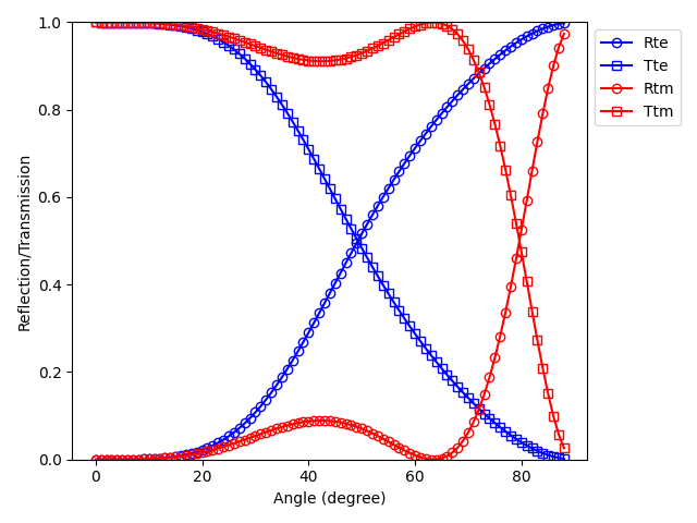
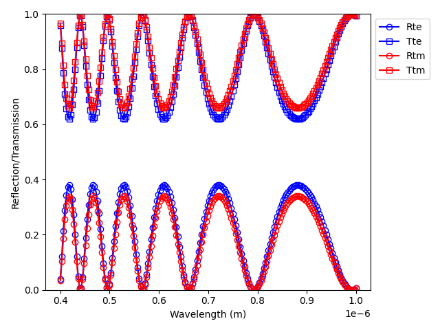
In the second set of calculation, we fix the angle of incidence and set up a spectral range over which we run the calculation:

theta = 15 ## fixed angle of incidence

lbda = np.linspace(400e-9,1e-6,200) ## 400nm to 1µm
f = c_const/lbda ## ferquency in SI units
f0 = f/c_const*1e-6 ## so the reduced frequency is f/c_const*a[SI units]

While the bulk of the code is the same, note that now we must remember to include the S.SetFrequency method in the main loop:

for ii, fi in enumerate(f0):
    S.SetFrequency(fi)
    ########
    ## TM excitation
    S.SetExcitationPlanewave(
            IncidenceAngles=(theta,0), #S4 names are reversed (phi,theta)
            sAmplitude=0.,
            pAmplitude=1.,
            Order=0)
    inc, r = S.GetPowerFlux(Layer='AirTop',zOffset=0)
    fw, _ = S.GetPowerFlux(Layer='AirBottom', zOffset=AirThick)
    Rtm[ii] = np.abs(-r/inc)
    Ttm[ii] = np.abs(fw/inc)

    #########
    ## TE excitation
    S.SetExcitationPlanewave(
            IncidenceAngles=(theta,0), #S4 names are reversed (phi,theta)
            sAmplitude=1.,
            pAmplitude=0.,
            Order=0)
    inc, r = S.GetPowerFlux(Layer='AirTop',zOffset=0)
    fw, _ = S.GetPowerFlux(Layer='AirBottom', zOffset=AirThick)
    Rte[ii] = np.abs(-r/inc)
    Tte[ii] = np.abs(fw/inc)

which quickly allows to plot the results:

Tutorial 3: Calculating absorption

Before moving to a more complex simulation, let’s apply the knowledge we have so far to extract a more subttle quantity from a simple simulation: the absorption of light inside a given layer. The example file is under examples/Absorption.py.

We set up a very basic 2D simulation, without any pattern, containing a superstrate, an absorbing slab and either a transparent or reflecting substrate:

f = 1 ## single frequency in reduced units
a = 1 ## period
S = S4.New(Lattice=a, NumBasis=1) ## Simple lattice

SlabThick = 2 ## thickness of absorbing slab
AirThick = 1 ## 0 should work also...

n = 3 ## slab index, real part
k = 0.01 ## slab index, imaginary part
epsSlab = (n+1.0j*k)**2 ## slab permittivity
epsMirr = -1e10 ## mirror, to mimic a metal

where a very large, real negative permittivity can be used to mimic a lossless metal. We will perform the computation at a single frequency but for several angles:

theta = np.arange(0,89,2)

and the slab is either surrounded by air or backed by a mirror:

S.SetMaterial(Name='Air', Epsilon=(1.0+1.0j*0))
S.SetMaterial(Name='Slab', Epsilon=epsSlab)
# S.SetMaterial(Name='Mirror', Epsilon=epsMirr)

S.AddLayer(Name='AirTop', Thickness=AirThick, Material='Air')
S.AddLayer(Name='Slab', Thickness=SlabThick, Material='Slab')
# either mirror or air for substrate
# S.AddLayer(Name='AirBottom', Thickness=AirThick, Material='Mirror')
S.AddLayer(Name='AirBottom', Thickness=AirThick, Material='Air')

The main loop looks similar to the previous simulations:

Rtm = np.empty(len(theta)) ## reflectivity
Ttm = np.zeros_like(Rtm) ## transmission
Atm = np.zeros_like(Rtm) ## absorption

for ii, thi in enumerate(theta):
    S.SetFrequency(f)
    S.SetExcitationPlanewave(
            IncidenceAngles=(thi,0), #S4 names are reversed (phi,theta)
            sAmplitude=0.,
            pAmplitude=1.,
            Order=0)
    inc, r = S.GetPowerFlux('AirTop', 0.)
    fw, _ = S.GetPowerFlux('AirBottom', 0.)
    Rtm[ii] = np.abs(-r/inc)
    Ttm[ii] = np.abs(fw/inc)
    fw1, bw1 = S.GetPowerFlux('Slab', 0)
    fw2, bw2 = S.GetPowerFlux('Slab', SlabThick)
    Atm[ii] = np.abs((fw2-fw1-(bw1-bw2))/inc)

The reflection and transmission are computed as always at the top and bottom boundary of the simulation. The three most important lines here are the last three:

fw1, bw1 = S.GetPowerFlux('Slab', 0)
fw2, bw2 = S.GetPowerFlux('Slab', SlabThick)
Atm[ii] = np.abs((fw2-fw1-(bw1-bw2))/inc)

where we store in fw1, bw1 the forward and backward power fluxed at the top boundary of the layer, and in fw2, bw2 the forward and backward power fluxed at the bottom boundary of the layer (note the zOffset parameter set at the value of SlabThick). Hence, the absorption in the layer is simply the difference between the in-flowing and out-flowing power. Thanks to the simple form of this simulation, we can quickly check the results:

where we plot the reflection and transmission. We compare the computed absorption (open symbols) to \(1-R-T\) (dashed line), and also check energy conservation (black dots). Using this, we are able to compute the absorption of light in any layer inside the simulation.

Tutorial 4: Dispersive Metal-Insulator-Metal grating

As a last tutorial, we focus on the optical properties of 1D rectangular metallic gratings under TM excitation. The example file can be found under examples/MIM_DispersiveGrating.py. This example demonstrates the first patterning method, and shows some of the more complex S⁴ options. In addition, it shows some of the utilities functions from S4Utils to make the python API more user friendly.

To install the S4Utils package, refer to the Download and installation section.

We import the necessary packages:

import time ## to time script execution
import S4 as S4
import numpy as np
import matplotlib.pyplot as plt

and two utility packages:

import S4Utils.S4Utils as S4Utils
import S4Utils.MaterialFunctions as mat

The first one contains various functions to facilitate the use of the S⁴ python API, while the second contains python defined permittivity functions. We will run the simulation over actual physical parameters, hence keeping track of the actual values of the frequency, lengths etc. Using micrometers as a base unit in the simulation we define the frequency range in the 12-50 THz range:

fmin = 12.0*1e12 ## 400cm-1 en Hz
fmax = 50.0*1e12
f = np.linspace(fmin, fmax, 200)
f0 = f/c_const*1e-6

We then define the unit cell using the period of the grating:

px = 3.6
ff = 0.8
s = ff*px
NBasis = 41
S = S4.New(Lattice = px,
        NumBasis = NBasis) ### NumBasis <=> halfnpw in RCWA

Here px is the simulation period, ff is the filling factor of the grating, and hence s is the size of the metal stripe.

Warning

As noted in various references, metallic gratings and more generally, high index contrast patterns, are generally difficult to model in RCWA. Hence, the number of Fourier coefficients to be considered has to be large to ensure a good convergence. Generally speaking, care must always be taken when setting the NumBasis parameter.

The reflectivity spectrum can be calculated for a single angle of incidence, or over a range of angles to get the dispersion relation of the grating modes:

theta = np.arange(0,90,5) ### for a dispersion plot
# theta = [0] ## for a single spectrum

We get the material permittivities from the Material database:

epsAu = mat.epsAu(f)
epsGaAs = mat.epsGaAs(f)

Note that contrary to the examples above, now we define dispersive materials, with a frequency-dependent permittivity. Hence, we store the value of the complex permittivity at each frequency of the simulation in an array. The permittivity of a material can also be defined as a tensor, e.g. with diagonal elements \(\varepsilon_x\), \(\varepsilon_y=\varepsilon_x\), \(\varepsilon_z\).

Note

The shape of the tensor can either be 3x3xlen(f) or len(f)x3x3

As we wish to use dispersive materials, we will need to update their permittivity each time the frequency of the simulation is changed. A utility function is available in S4Utils to take care of this for all dispersive materials in the simulation: S4Utils.S4Utils.UpdateMaterials(), which we will use later in the script.

The materials are set as usual, and we initialize the dispersive materials with the first value of the permittivity array:

DisplayThick = 0.5 ## Incident medium thickness
ARThick = 1.0 ## Active region thickness
AuThick = 0.1 ## Gold thickness

### Materials
S.SetMaterial(Name='Air', Epsilon=(1.0 + 0.0*1.0j))
S.SetMaterial(Name='Au', Epsilon=(epsAu[0]))
S.SetMaterial(Name='AR', Epsilon=(epsGaAs[0]))

In order to use the function that updates the dispersive materials permittivities, we need to store the material names and permittivity tensors in two lists:

# material list for the update function
Mat_list = ['Au', 'AR']
Eps_list = [epsAu, epsGaAs]

We then add the layers to the simulation:

### Layers
S.AddLayer(Name='top', Thickness = DisplayThick, Material = 'Air') ## incident medium, air
S.AddLayer(Name='TopGrating', Thickness = AuThick, Material = 'Air') ## grating layer, will be patterned
S.AddLayer(Name='AR', Thickness = ARThick, Material = 'AR') ## active region layer
S.AddLayer(Name='Bulk', Thickness = 2*AuThick, Material = 'Au') ## bottom mirror

Now we need to specify the patterning of the TopGrating layer (see the S.SetRegionRectangle function):

### Geometry
S.SetRegionRectangle(
    Layer='TopGrating',
    Material='Au',
    Center=(0.0,0.0),
    Angle=0.0,
    Halfwidths=(s/2.,0)) # 1D

The patterning method takes the layer to be patterned as an argument, and the material in which the pattern should be made. Note also that since this is a 2D simulation, the halfwidth of the pattern is s/2 along the patterning direction, and 0 in the transverse direction.

Before running the simulation, a few additional options have to be set:

### Simulation options
S.SetOptions(
    Verbosity=0, ## verbosity of the C++ code
    DiscretizedEpsilon=True, ## Necessary for high contrast
    DiscretizationResolution=8,  ## at least 8 if near field calculations
    LanczosSmoothing = True, ## Mabe ?? especially for metals, for near fields
    SubpixelSmoothing=True, ## definitely
    PolarizationDecomposition=True, ## Along with 'normal', should help convergence
    PolarizationBasis='Normal')

Description of theses options are available in the RCWA formulations and S.SetOptions documentations. A priori, evaluation of the Fourier coefficients of the permittivities for anisotropic materials requires discretization of the permittivity patterns, hence we always set the DiscretizedEpsilon=True flag to compare simulations run with the same RCWA formulation. The other options improve the convergence with high refractive index contrast, and the spatila resolution of fields computed in each layers.

The simulation now consists in two nested loops:

R = np.empty((len(theta),len(f)))

ProgAngle = 0 ## progress in angle sweep
for ii, thi in enumerate(theta): ## angle sweep
    currAngle = int((ii*10)/len(theta)) ## current angle by 10% steps
    if currAngle>ProgAngle:
        print(currAngle) # print progress every 10%
        ProgAngle = currAngle
    ProgF = 0  ## progress in frequency sweep
    for jj, fj in enumerate(f0):  ## frequency sweep
        currF = int((jj*10)/len(f0)) ## current frequency by 10% steps
        if currF>ProgF:
            print('\t %d'%currF) # print progress every 10%
            ProgF = currF

        S.SetFrequency(fj)  # set the current frequency
        S4Utils.UpdateMaterials(S, Mat_list, Eps_list, fj, f0) # set epsilons
        S.SetExcitationPlanewave(
                IncidenceAngles=(thi,0.),
                sAmplitude=0.,
                pAmplitude=1.,  ## p-pol plane wave
                Order=0)
        inc, r = S.GetPowerFlux('top', 0.)
        R[ii,jj] = np.abs(-r/inc) ## reflectivity

At each loop step, it is crucial to ensure that three main operations are performed: Setting the simulation frequency:

S.SetFrequency(fj)  # set the current frequency

Updating the dispersive materials permittivities using the previously defined Mat_list and Eps_list lists defined previously:

S4Utils.UpdateMaterials(S, Mat_list, Eps_list, fj, f0) # set epsilons

and finally ensuring that the excitation is performed with the correct angle and polarization:

S.SetExcitationPlanewave(
        IncidenceAngles=(thi,0.),
        sAmplitude=0.,
        pAmplitude=1.,  ## p-pol plane wave
        Order=0)

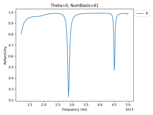
Finally, we plot the results, either for a single spectrum or for a dispersion relation:

if len(theta)==1:
    figsp = plt.figure()
    ax = figsp.add_subplot(111)
    ax.plot(f, R.T)
    ax.set_xlabel('Frequency (Hz)')
    ax.set_ylabel('Reflectivity')
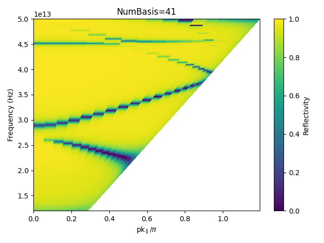
else:
    figdisp = plt.figure()
    axm = figdisp.add_subplot(111)
    thm, fm = np.meshgrid(theta,f)
    km = (px*1e-6)*(2*np.pi*fm)/c_const*np.sin(np.deg2rad(thm))/np.pi
    cax = axm.pcolormesh(km, fm, R.T,
                        vmin=0, vmax=1,
                        shading='None')
    axm.set_xlabel('pk$_{\parallel}$/$\pi$')
    axm.set_ylabel('Frequency (cm$^{-1}$)')
    figdisp.tight_layout()
plt.show()

which leads e.g. for a normal incidence:

or a dispersion with a 5° step which runs in around one minute on a laptop:

Having computed the spectum, we might want to look at the field distribution in the structure. The python API directly provides some functions to compute the electric field from a given simulation, especially S.GetFields and S.GetFieldsOnGrid. The first one computes the electric and magnetic field tensors at a single given point in space, while the second computes the electric and magnetic fields tensors on an \(x-y\) coordinate. This function thus only returns correct values in 3D simulations. To make the computations and visualizations easier, S4Utils provides a set of functions to extract electric and magnetic field profiles along slices (Simulation Functions) and plot them in a practical visualization environment (S4Utils Plotting Utilities). Additionally, it also provides a way to extract the reconstructed permittivity profile using S.GetEpsilon, to help extract an image of the geometry, which can sometimes be hard to picture. This also provides a sense of the spatial resolution of the permittivity decomposition.

Say we want to visualize the profile of the vertical component of the electric field at the 28.8 THz resonance upon normal incidence excitation. We set up the simulation:

fplot = 28.8e12 ## frequency at which we plot (SI)
f0plot = fplot/c_const*1e-6 # reduced units
S.SetFrequency(f0plot)
S4Utils.UpdateMaterials(S, Mat_list, Eps_list, f0plot, f0) # update materials
S.SetExcitationPlanewave(
    IncidenceAngles=(0.,0.), ## normal incidence
    sAmplitude=0.,
    pAmplitude=1.,  ## p-pol plane wave
    Order=0)

and define the grid coordinates on which we want to extract the field:

resx = 150 ## x-resolution
resz = 150 ## z-resolution
x = np.linspace(-px/2, px/2, resx) ## x coordinates
z = np.linspace(0, TotalThick, resz) ## z coordinates

Here we choose to plot the field on a single period, however since S⁴ takes care of the periodicity by itself, we could have set arbitrary values for the x-coordinates and plot over several periods. Since this is a 2D simulation, we have to use S.GetFields and loop over each coordinate points. This is well take care of by S4Utils.S4Utils.GetSlice():

E, H = S4Utils.GetSlice(S, ax1=x, ax2=z, plane='xz', mode='Field')
FigEz = S4Utils.SlicePlot(x, z ,np.real(E[:,:,2]), hcoord=s/4)
FigEz.ax_2D.set_ylabel('z')
FigEz.ax_2D.set_xlabel('x')
FigEz.axcbar.set_ylabel('Ez')

Here the calculation is performed by S4Utils.GetSlice(S, ax1=x, ax2=z, plane='xz', mode='Field') where we pass the simulation object S as an argument, along with the vector of coordinates x and z. The plane keyword (one of xy,yz,xz) indicates which coordinates to loop over in the C++ function, and the mode keyword allows to compute only the fields (Field), the permittivity (Epsilon) or both (All). E and H are len(x)*len(y)*3 arrays containing the complex electric and magnetic field amplitude. Hence, the vertical component of the electric field is simply np.real(E[:,:,2]). It could be plotted using a simple plt.pcolormesh or plt.imshow, however S4Utils provides a simple visualization tool that allows to plot fields and slices using S4Utils.S4Utils.SlicePlot():

FigEz = S4Utils.SlicePlot(x, z ,np.real(E[:,:,2]), hcoord=s/4)

which is a simple class wrapping around a matplotlib figure instance, and hence can be customized after creation such as changing labels:

FigEz.ax_2D.set_ylabel('z')
FigEz.ax_2D.set_xlabel('x')
FigEz.axcbar.set_ylabel('Ez')

Which allows us to get the 2D electric field plot below, with a symmetrized blue-white-red colormap.

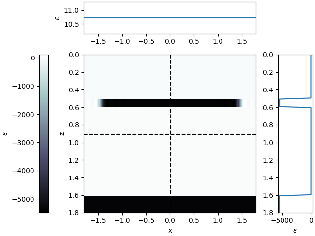
We do the same for the permittivity profile, showing also some more customization options for the SlicePlot class:

Eps_plot = S4Utils.GetSlice(S, ax1=x, ax2=z, plane='xz', mode='Epsilon')
FigEps = S4Utils.SlicePlot(x, z, np.real(Eps_plot), cmap=plt.cm.bone,
                        sym=False)
FigEps.ax_2D.set_ylabel('z')
FigEps.ax_2D.set_xlabel('x')
FigEps.axcbar.set_ylabel(r'$\varepsilon$')

and plot the permittivity profile: